Nonparametric Confidence Intervals
Mathematics | . Edited . 10 min read (2443 words).


Implementation guide for calculating nonparametric confidence intervals of the population mean based on the Dvoretzky–Kiefer–Wolfowitz inequality.
Topics:
Introducing the example model
 This blog post will focus on the following
specific example scenario based on product ratings. Generalisation from this is
discussed later.
This blog post will focus on the following
specific example scenario based on product ratings. Generalisation from this is
discussed later.
Assume that a website allows users to rate products or similar (such as books on goodreads) by giving the product an integer rating between 1 and 5. Furthermore, assume that users have a fixed taste over time and that the users who actually entered their ratings are drawn from the population of all applicable users uniformly randomly. Furthermore, assume that there’s an infinite population of users instead of having a known finite number.
This is not entirely realistic, but leads to a simple statistical model that can be used to calculate a reasonable confidence interval for the average rating of all users based on the sample of ratings we have received at the moment. All we need to calculate this is the count of ratings at each rating level and the desired confidence level of the interval.
Nonparametric model and validity
The model described above is nonparametric in the sense that it doesn’t make any assumptions about the statistical distribution itself. It still makes an assumption that ratings are IID (independent and identically distributed) and that the total population is unbounded. This is unlikely to be fully true, but offers a simplifying approximation that is likely to be sufficient in many cases. By making minimal assumptions, the model is widely applicable (at least approximately).
An example of a situation where the model’s assumptions wouldn’t be valid is when a product gets widespread publicity (such as a movie adaptation) and ratings of readers before and after this are distributed differently. Such a change in rating distributions would introduce some bias and result in the confidence interval being overly confident directly after the change. Another potential reason for a change in distribution over time is that early raters are either more positive or more critical than mainstream raters who add their ratings later.
Another assumption that is unlikely to be fully valid ever is the infinite population. This is a reasonable approximation of reality in many situations, but not for products with limited copies. Imagine a bespoke product that will only ever be available in 10 copies. When we have 10 ratings, we know the exact average rating for the entire population and the statistical model above will overestimate the uncertainty since it doesn’t know that further ratings are impossible.
It would be possible to take for example time into consideration and possibly reduce bias, but this would introduce more variance and allow us to draw weaker conclusions based on the same amount of data. This is the classic bias-variance tradeoff that shows up in statistics and machine learning. In general, a bound on the population size won’t be available and is not useful to incorporate into the model for that reason.
Interactive demonstration
You can enter data in the following input fields to calculate confidence intervals interactively based on the above example:
Confidence level (%):
Number of ratings: 1: 2: 3: 4: 5:
Confidence interval for average rating: .
What is a confidence interval?
A confidence interval is a special case of a confidence set. A confidence set is a way to estimate a parameter of a distribution based on a sample of data from the distribution. It does this at a certain confidence level by computing a set from the sample data such that this set will cover the true parameter value with a probability equal to or higher than the confidence level.
Slightly more formally, a confidence set $C_n$ for a parameter $\theta$ of a probability distribution at the confidence level $1 - \alpha$ is any function of a random sample from the distribution with $n$ data points to a set of possible values for $\theta$ that fulfils the following:
$$\mathbb{P}(\theta \in C_n) \geq 1 - \alpha,$$for all $\theta$. Note both that $C_n$ is a function of the random sample and that $\theta$ is the true value of the distribution parameter. $\theta$ is fixed and $C_n$ is random. The probability is in relation to drawing random samples and calculating confidence sets based on the sample.
What this means is that when we draw a new random sample and calculate a confidence set using a predetermined function with a confidence level of $1 - \alpha$, there’s at least a probability of $1 - \alpha$ that the confidence set will cover the true parameter value.
Importantly, it’s a probability statement about the confidence set and not the parameter (which is fixed). It does not mean that there’s a probability of $1 - \alpha$ that $\theta$ is within a specific confidence set. It either is or isn’t. It’s only when we see the confidence set as a random variable that the probability statement makes sense and it refers to the confidence set.
On a large website with many product ratings, we can for example correctly assume that if we randomly pick one product and look at its confidence interval, it will be correct (i.e. contain $\theta$) with a probability of approximately $1 - \alpha$. This gives an indication of how many of the confidence intervals are wrong. Note that some confidence intervals will be wrong and they are fully allowed to be wildly wrong.
The above definition isn’t the only possible and it describes conservative confidence intervals. It’s also common with approximate confidence intervals and it’s possible to instead require that the probability is exactly $1 - \alpha$ to get exact confidence intervals.
One important property of confidence intervals is that they are typically not unique. What we’re looking for is one function that generates valid confidence intervals for a distribution. We’re not looking for the one and only.
Dvoretzky–Kiefer–Wolfowitz inequality
To construct a nonparametric confidence interval, we will use the Dvoretzky–Kiefer–Wolfowitz (DKW) inequality. The mathematical details are described both on Wikipedia and in the book All of Statistics by Larry Wasserman and many other statistics books.
The goal of this blog post isn’t to delve into the mathematical details, but an overview follows here. What is important in the following is the calculation of $\epsilon$ based on $\alpha$ from the confidence level (commonly $\alpha = 0.05$) and the number of data points $n \geq 0$. The definition of a CDF is given further down.
Theorem: The Dvoretzky-Kiefer-Wolfowitz (DKW) Inequality. Let $F$ be a cumulative distribution function (CDF) and $F_n$ be the empirical CDF based on a sample of size $n$ from the same distribution. Then, for any $\epsilon > 0$,
$$\mathbb{P}\left( \sup_x |F(x) - F_n(x)| > \epsilon \right) \leq 2e^{-2n\epsilon^2}.$$The DKW inequality provides an upper bound on the probability that the empirical CDF deviates more than $\epsilon$ from the true CDF at any point.
Info: Supremum. For anyone unfamiliar with supremum, the $\sup_x$ in the DKW inequality means supremum over all $x$ and is a concept from mathematical analysis that can be thought of as the maximum value. It means approximately the maximum value of $|F(x) - F_n(x)|$ over all possible $x$. Supremum is a little more flexible, however, since it’s possible that no maximum value is actually achieved and supremum still has a well-defined meaning.
An alternative way to write the above is:
$$\mathbb{P}\left(|F(x) - F_n(x)| > \epsilon, \text{ for any } x\right) \leq 2e^{-2n\epsilon^2}.$$Info: Absolute value. Another important part of the DKW inequality is $|x|$, which is the absolute value of x, defined as:
$$ |x| = \begin{cases} x &\text{if }x \geq 0\newline -x &\text{otherwise} \end{cases} $$The absolute value can be thought of as removing any minus sign. In this situation, it is used to calculate the absolute difference between two values (i.e. the unsigned distance between them when disregarding which is bigger).
From this, we can draw some conclusions about the opposite too:
\begin{gather*} \mathbb{P}\left( \sup_x |F(x) - F_n(x)| \leq \epsilon \right) = \newline = 1 - \mathbb{P}\left( \sup_x |F(x) - F_n(x)| > \epsilon \right) \geq 1 - 2e^{-2n\epsilon^2}. \end{gather*}
This suggests a way to create a confidence set, since it’s starting to look like the definition of a confidence set above. What $\epsilon \geq 0$ do we need to get $1 - \alpha$ on the right hand side? Let’s see:
\begin{align*} 1 - \alpha &= 1 - 2e^{-2n\epsilon^2} \newline \Leftrightarrow \quad \alpha &= 2e^{-2n\epsilon^2} \newline \Leftrightarrow \quad \ln(\alpha/2) &= -2n\epsilon^2 \newline \Leftrightarrow \quad \ln(2/\alpha) &= 2n\epsilon^2 \newline \Leftrightarrow \quad \epsilon &= \sqrt{\frac{1}{2n} \ln \frac{2}{\alpha}} \end{align*}
This assumes $\epsilon \geq 0$, since that’s the only allowed value in the original DKW inequality above.
Info: Equivalence. The symbol $\Leftrightarrow$ is used above to mean is equivalent to. $A \Leftrightarrow B$ indicates that A and B are mathematically equivalent statements. What this means is that A and B are either both true or both false. Another way of saying this is that B is true iff (if and only if) A is true.
Above, each equation is equivalent to the other equations (under the assumption that $\epsilon > 0$), which means that the exact same set of variable values satisfy all of them. Loosely speaking, they are all interchangeable as they have the exact same underlying meaning.
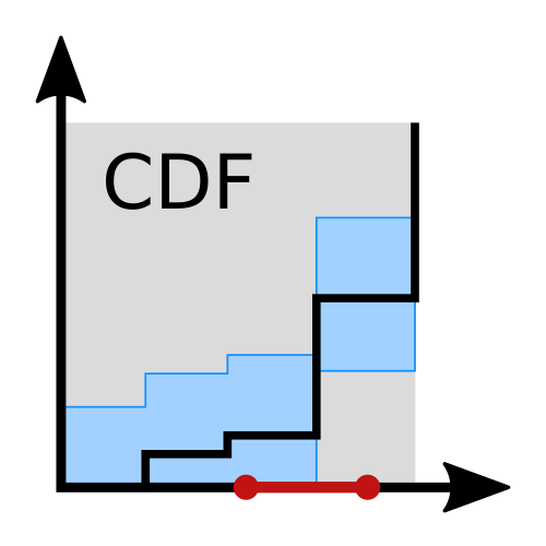
Given $\epsilon$ as calculated here, we can construct a simultaneous confidence band vertically centred around the empirical CDF with width $2\epsilon$ (i.e. $\epsilon$ distance both straight upwards and downwards) and it will cover the real CDF in all points with at least $1-\alpha$ probability.
CDF confidence band
Based on the theory above, we can construct a CDF confidence band as follows.
\begin{align*} \epsilon &= \sqrt{\frac{1}{2n} \ln \frac{2}{\alpha}} \newline U(x) &= \min\{{F_n(x) + \epsilon, 1\}} \newline L(x) &= \max\{{F_n(x) - \epsilon, 0\}} \newline \end{align*}
Here, the confidence band is between $U(x)$ and $L(x)$ and it follows that:
$$\mathbb{P}(L(x) \leq F(x) \leq U(x) \text{ for all } x) \geq 1 - \alpha.$$This can be graphed to illustrate it further, but instead we’ll discuss how to apply this to calculate a confidence interval for the average.
Calculate the expected value from a CDF
The expected value is also known as the mean or average. For our purposes here, it’s sufficient to calculate the expected value of a discrete CDF such as the empirical CDF.
Definition: cumulative distribution function (CDF). The CDF of a random variable $X$ is given by:
$$F(x) = \mathbb{P}(X \leq x).$$For a discrete probability distribution, the CDF is piecewise constant with discontinuities only at the possible values of the distribution. Here, it’s sufficient to assume that the possible values are finite even.
Let $X$ be distributed according to a finite discrete probability distribution with CDF $F$ and let all the possible values be $x_1, x_2, \dots, x_n$. The expected value of $X$ is then
$$E[X] = \sum_{i=1}^n x_i \mathbb{P}(X = x_i) = x_1 F(x_1) + \sum_{i=2}^n x_i (F(x_i) - F(x_{i-1})).$$This can be applied to $U(x)$ and $L(x)$ almost directly. However, there is one small modification we need to make to these bounds to turn them into proper CDFs. For the highest possible value $x_n$, we need $F(x_n) = 1$. This is not necessary when they are just bounds, but for a CDF we know that it will be 1 for the highest possible value and also it needs to achieve 1 at its maximum value to be a valid CDF. On the lower end, this works out nicely by itself.
Given this tiny modification, we can calculate the expected value of these CDFs related to $U$ and $L$.
Confidence interval for the expected value
We have almost all the necessary building blocks now, but one piece is missing. How do we go from the confidence band to a confidence interval for the expected value of the ratings (the average)? We can directly use the simultaneous confidence band for this. Since it covers the entire real CDF by the correct probability, we just need to figure out what upper and lower bounds this band puts on the expected value we’re after.
Proving this result formally might be a bit tricky, but it’s intuitively easy to see that the $L(x)$ function (adjusted to become a CDF) results in the highest possible expected value of any CDF inside the confidence band and the opposite for $U(x)$.
This gives us the following lower bound on the expected value:
$$ I_0 = x_1 U(x_1) + x_n (1 - U(x_{n-1})) + \sum_{i=2}^{n-1} x_i (U(x_i) - U(x_{i-1})). $$The upper interval bound is given by:
$$ I_1 = x_1 L(x_1) + x_n (1 - L(x_{n-1})) + \sum_{i=2}^{n-1} x_i (L(x_i) - L(x_{i-1})). $$The $1- \alpha$ confidence interval of the expected value is given by $(I_0, I_1)$ (an interval between these values). This is a function of the sample. See the definitions of $1 - \alpha, \epsilon, U(x), L(x)$ above. It’s important that the set of possible values $\{{x_i\}}$ contains the biggest and smallest possible values even if neither was observed yet, since they both affect the confidence interval. The other values $x_i$ can in theory be kept to only those with non-zero frequencies in the sample.
When only a single possible value exists, the interval trivially consists of only that value instead: $(x_1, x_1)$. The situation where no known range of possible values exists makes little sense to calculate confidence intervals for on the other hand.
To summarise what data is needed, it’s this: minimum and maximum possible values, confidence level ($1 - \alpha$), and observed values with frequencies (i.e. counts). It’s possible to write very generic source code to calculate the above type of confidence interval for the expected value based only on this.
Example JavaScript library
For a full implementation with some unit tests, see my dkw-confidence-intervals-js project on GitHub. It’s open source and can be used directly. It only calculates confidence intervals for the expected value, but could be extended to calculate other similar confidence intervals.
Final notes
I hope that it’s reasonably easy to implement this specific type of nonparametric confidence intervals and interpret them based on this blog post. Have a look at the example code to fill in any gaps in the description!
Personally, I hope confidence intervals like this would show up on websites for product ratings and any similar data. Choosing a classic 95% confidence level is a safe initial choice for anyone unsure. That will make it quite rare that users encounter incorrect confidence intervals, but it’s still important to specify the confidence level as a confidence level of 100% is useless (try it above!).